“I need math assistance!”
Few words make me more willing to drop everything else I’m doing at work and hear out a colleague’s problems. Recently that is exactly the Teams chat I received at 4:43 pm.
“I live for these moments,” I responded, only half-joking.
The problem was this: If we know that our fare checkers ask x percent of light rail passengers each day for proof that they paid their fare, how long would a passenger expect to ride before they get fare checked?
Approaching the Problem
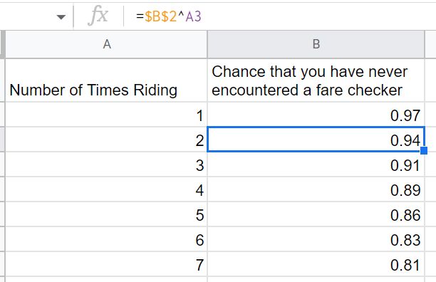
Here’s a way to think about this problem. Let’s say we know that on any given ride, you have a 3% chance of getting fare-checked. That means that you have a 97% chance of not getting fare checked. So after one ride, there’s a 97% chance that you have never encountered a fare checker.
Now you ride a second time. You again have a 97% chance of not encountering a fare checker on this particular ride (and every ride thereafter). So your chance of not encountering a fare checker either your first or second time is now 97% times 97%, or 94.1%. Intuitively, this number will go down the more you ride: It’s easy to go one ride without getting checked, but it’s a lot harder to go 10 or 50 rides.
What I’m wanting to know here is at what point those odds go down to 50%. At what point would it start to be a little remarkable that I have ridden a lot and still not seen a fare checker?
The Long Way
You can do this manually in Excel pretty simply and it may help you to grasp what is happening here. You are taking the chance of not seeing a fare checker and raising it to the power of how many times you have ridden.
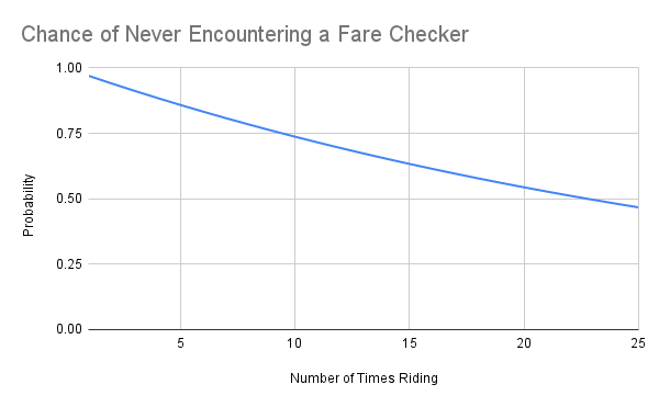
If you continue this down a few more rows, you’ll see that it reaches 0.5 between the 22nd and 23rd ride. That’s a long time! Here’s that in a more visual form. You can see the plot crossing the y = 0.5 line at around x = 22.
In statistics, these numbers can be generated by the geometric distribution. Given a probability x of a given event (such as probability 0.03 of getting fare checked on any given ride), the geometric distribution can tell you how many trials you would expect to take before the event happens. It can also tell you how many M&Ms you would eat before finding one that is disfigured or how many clovers you would look through before finding one that has four leaves, as long as you know how often those things happen overall. Critically, these have to be independent events where the chance of it happening is always the same. In this example, my chance of getting fare checked on any given ride does not waver. It is always 3%, whether I just got fare checked this morning or haven’t been checked in a year. Yesterday’s events don’t affect today’s.

The short way
I’m always a fan of doing something the long way the first time so I really get it. But when you’re ready to save time, you can solve this problem in R more quickly and succinctly using the qgeom function. My inputs are 0.5 (because I am interested in when my odds of never encountering a fare checker get down to 50%) and .03, my chance of encountering a fare checker on any given ride.
The resulting 22 matches what we got in Excel: Given a 3% fare checking rate, I could ride 22 times and there would still be a 50% chance that I would never have encountered a fare checker.
By changing the 0.03 in the above code to something else, I can also quickly model how this would change if fare checks ramped up or down. For example, if policies changed and 10% of people were checked on any given day, then I’d expect to see a fare checker a lot sooner (after only 6 rides, in fact).
So, how much does the check rate matter? If you want people to feel like there’s a reasonable chance they’ll get checked, then increasing your check rate helps, but there are diminishing returns: it makes a big difference to go from a very low to low rate of fare checking, but it matters less to go from a high to very high rate. Here’s how long you’d expect to go before getting checked given different fare check rates.
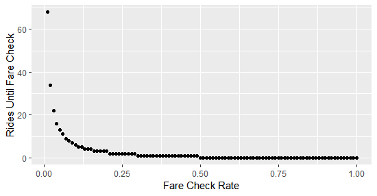
So going from a 1% to 3% rate dramatically cuts down on the number of times I can expect to ride before getting fare checked. Going from 25 to 28% has nowhere near the same effect.
But wait…
You might be wondering: If I I have a 1% chance of getting checked on a given trip (meaning I get checked one in every 100 trips), then wouldn’t I just expect to go 50 trips before my first encounter, since that is half of 100? Why does the graph above tell me it’s over 60?
The reason that the answer is 68 rides and not 50 in that scenario is that seeing a fare checker on any given ride is an independent event. The fact that I got checked yesterday in no way makes me more or less likely to get checked today. In fact, I could in theory ride my whole life and by extreme luck, never get fare checked.
Compare that to something like guessing the code on a combination lock.
If there are 100 possible combinations and you start guessing them in order, then eventually you will have to find the combination. Each time you guess incorrectly, your chance of being correct the next time increases because there are fewer options left. So you would expect, on average, to find the combination after 50 tries on average and you are guaranteed to take 100 tries or less. Not so with an independent event like a fare check.
You can use the geometric distribution to model other independent events in transportation (if assumptions are met), such as: counting users of a bike trail until you find someone on an e-bike; number of days before a bus’s windshield gets chipped; or number of flights before a passenger’s luggage gets lost.
I hope you enjoy using the geometric distribution and qgeom to explore probability!
